

What is a VLOOKUP, and why does it show up in almost every Excel tutorial? It is a formula that finds a value in one table and pulls back matching data from another column in that same row.
The first spreadsheet where I needed it was a payroll file: employee IDs lived in one tab, salaries in another, and VLOOKUP was the fastest way to line them up.
VLOOKUP Excel formulas solve one everyday problem: two tables that need to talk to each other. Below, you will see what each part means, real examples you can copy into your own sheet, common errors, and when a newer function like XLOOKUP works better for the job.
What is a VLOOKUP in Excel?
VLOOKUP stands for vertical lookup. It searches the left column of a range for a value, then returns matching data from another column in that row.
Say you have an employee ID in one sheet and need the matching email in another. VLOOKUP finds it in one step, instead of scanning row by row.
The function has been part of Excel for decades, which is why payroll sheets and sales reports still lean on it every day. I still open decade-old templates at client sites that use nothing but VLOOKUP, mainly because it works in every version of Excel without needing an add-in.
Anyone opening a VLOOKUP Excel formula for the first time is usually solving a simple matching task, such as finding related information from a table. Microsoft’s VLOOKUP documentation covers how the function works, its syntax, and common uses.
Understanding the VLOOKUP Formula and Its Four Arguments
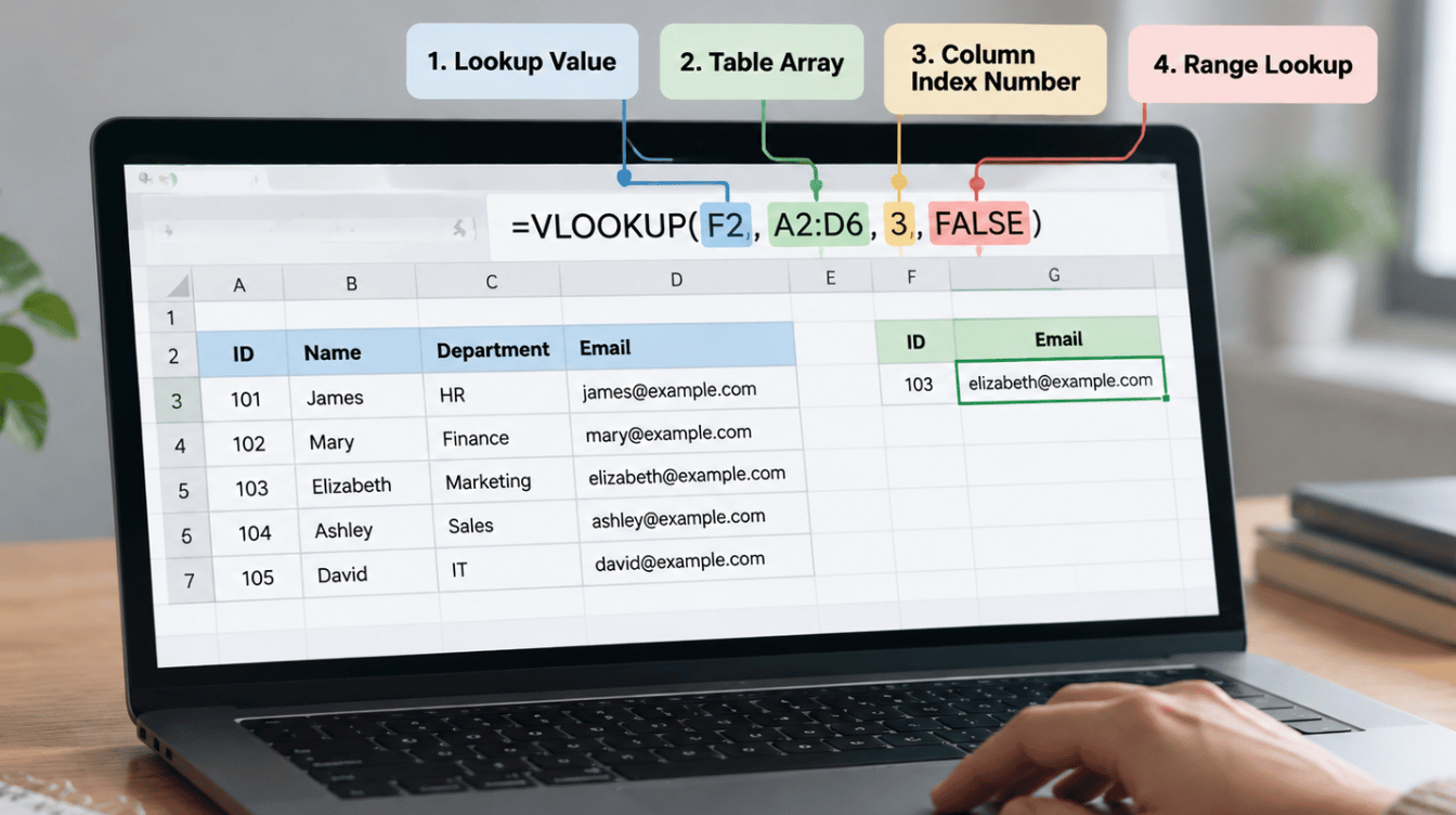
Every VLOOKUP formula uses four parts, always in the same order. Learn what each part controls, and the rest of this formula gets much easier to write on your own.
1. Lookup Value
The lookup_value is what Excel searches for. It is usually a cell, not typed text. In a payroll sheet, this might be an employee ID in column A. In a sales report, it could be a product code in column B. Excel checks the first column of your range for a match.
A stray space, a typo, or the wrong data type breaks the search right away, before the rest of the formula even runs. I have lost real time to a single trailing space in a lookup value more than once.
2. Table Array
The table_array is the full block of cells Excel searches. It must start with the column that holds your lookup value.
A common mistake is picking a range that starts one column too far right. This quietly breaks the whole formula. Lock the range with dollar signs, like $D$2:$G$10, so it stays fixed when you copy the formula down.
Get this right the first time, since most VLOOKUP errors trace back to the wrong table array. The same discipline pays off well beyond spreadsheets; it’s the same instinct behind picking the right tool for keeping any team’s work organized.
3. Column Index Number
The col_index_num tells Excel which column holds your answer. It counts from the left edge of the table array, not the worksheet itself.
If your range starts at column D, then D is one, E is two, and so on. Beginners often confuse this count with real worksheet letters. That mix-up pulls results from the wrong field. Adding or removing a column inside the range can shift this number without any warning.
4. Range Lookup
The range_lookup argument sets the match type. Type FALSE for an exact match. Use this for IDs, emails, or codes where close isn’t good enough.
Type TRUE for an approximate match. This works for sorted data, like tax brackets or commission tiers. Skip this argument, and Excel defaults to TRUE.
That quiet default causes wrong results on data that was never sorted in the first place, so type it on purpose every time.
Prepping Your Data Before You Build a VLOOKUP
Most VLOOKUP problems start before you even write the formula. A few habits catch them early:
- Keep the lookup column free of duplicate values, or VLOOKUP will return only the first match it finds.
- Match data types across both tables. A product code stored as text in one sheet and as a number in the other will not match, even when the values look identical.
- Convert a raw range into an Excel Table with Ctrl+T, so the reference expands automatically as rows are added, instead of needing to be redrawn.
- Name the lookup range something readable, such as EmployeeList, so the formula stays clear and correct even if you insert rows above it.
These habits take a few minutes now, but they save far more later, in much the same way automating repetitive tasks upfront saves a team from repeating manual work down the line.
How to Use VLOOKUP in Excel: Step by Step
Reading about VLOOKUP only goes so far. Building one formula on a real dataset is what makes it click. The steps below use a simple employee lookup table as the working example.
- Set up a source table and a lookup table.
- Click the cell for the result.
- Type =VLOOKUP( to begin.
- Select the lookup value.
- Select the table array.
- Enter the column index number.
- Type FALSE or TRUE.
- Close and press Enter.
Once the formula returns the right result on one row, copy it down the column. It applies the same logic to every remaining row, with no retyping needed at all.
The habit that saves the most time is pressing F4 right after selecting the table array. It locks the range with dollar signs before you even copy the formula down, which is the step most beginners forget until the formula breaks. Small shortcuts like this can matter as much as the tools built to save time elsewhere in your day.
Real-World Examples of VLOOKUP Formulas
Textbook examples rarely look like the spreadsheets people use at work. These scenarios show up often in payroll, retail, and customer service sheets at small and mid-sized US businesses. Each one takes just seconds to run.
- Find an employee’s email from their ID:
=VLOOKUP(A2,EmployeeList,3,FALSE) - Find a product’s price from its name:
=VLOOKUP(B2,PriceList,2,FALSE) - Find a letter grade from a numeric score:
=VLOOKUP(C2,GradeScale,2,TRUE) - Match a customer record between two sheets:
=VLOOKUP(D2,Sheet2!A:D,4,FALSE) - Pull a tax rate from an income bracket table:
=VLOOKUP(E2,TaxBrackets,2,TRUE)
The range name and column number change in each one, but the shape of the formula never does, which is what makes VLOOKUP worth memorizing once and reusing everywhere.
Common VLOOKUP Errors and How to Fix Them
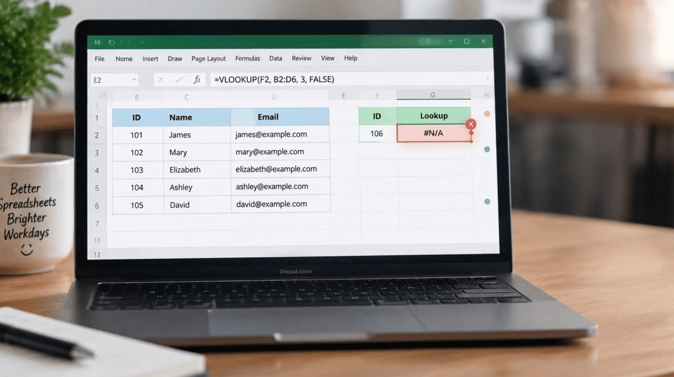
Most VLOOKUP problems come from a short list of repeat causes, not dozens of unrelated issues. Spotting the pattern behind each error cuts your troubleshooting time down fast, even on a messy shared file.
|
Error or Issue |
Likely Cause |
How to Fix It |
|---|---|---|
|
#N/A error |
Missing or misspelled value |
Check spelling and trailing spaces |
|
Wrong result |
TRUE used, unsorted data |
Switch to FALSE |
|
Breaks when copied |
Reference not locked |
Lock the range with dollar signs |
|
Only first match shows |
Duplicate values |
Add a helper column |
|
Text stored as numbers |
Data types don’t match between sheets |
Convert with VALUE() or reformat the column |
Most fixes take a minute or two once you spot the real cause. That beats deleting the whole formula and starting over. Microsoft’s own guide to #N/A errors covers more edge cases in detail.
VLOOKUP Limitations Worth Knowing
VLOOKUP handles simple lookups well, but it was never built to cover every case that comes up in a real spreadsheet. A few limits are worth knowing before you lean on it for bigger, more complex projects at work.
- It only searches the leftmost column of the selected range.
- It can only return values located to the right of that column.
- Inserting or deleting a column inside the range can shift the column index number without warning, which is one more reason to build the range as a named Table rather than a plain cell reference.
These limits do not make VLOOKUP unreliable for daily use, and most users never hit all three at once. They are also the exact reason Excel eventually shipped XLOOKUP.
VLOOKUP Best Practices for Cleaner Spreadsheets
A working VLOOKUP and a reliable one aren’t always the same. A few habits keep formulas from breaking as a workbook grows:
- Wrap the formula in IFERROR, such as:
=IFERROR(VLOOKUP(A2,EmployeeList,3,FALSE),"Not found"), so a missing match shows a clear message instead of #N/A. - Lock the table array with dollar signs or a named range before copying the formula down or across.
- Avoid nesting one VLOOKUP inside another on large datasets. Each nested lookup rescans the full range, and on sheets with tens of thousands of rows, that adds up to a noticeably slower recalculation.
- Sort the lookup column only when using an approximate match (TRUE). Sorting a column meant for exact matches (FALSE) buys nothing and risks reordering data that other formulas depend on.
Our list of Excel formula shortcuts has a few more time-savers worth pairing with these.
On a sheet with more than a few thousand rows, these small habits are usually what separates a formula that still works in six months from one that quietly breaks.
VLOOKUP Excel Alternatives: XLOOKUP and INDEX MATCH
VLOOKUP’s limits start to matter more on bigger projects with messier data. Two other Excel functions solve the same problem with fewer restrictions. Once a workbook outgrows a few hundred rows, this is usually where I start pointing people toward one of the two options below.
|
Feature |
VLOOKUP |
XLOOKUP |
INDEX MATCH |
|---|---|---|---|
|
Searches left or right |
No, right only |
Yes, either direction |
Yes, either direction |
|
Exact match by default |
No |
Yes |
Depends on setup |
|
Affected by inserted columns |
Yes |
No |
No |
|
Learning curve for beginners |
Easier |
Moderate |
Slightly higher |
XLOOKUP now ships with Excel 365 and Excel 2021, though older versions like Excel 2019 do not include it. Microsoft’s own XLOOKUP documentation calls it the more flexible pick for large or changing datasets. Plenty of teams stay on VLOOKUP anyway, usually because every past version of the workbook already used it.
Summing It Up
Now that you know what a VLOOKUP is, the four arguments are the real skill worth practicing on data that matters to you, not a sample table from a tutorial.
The version I still reach for daily is the exact FALSE match, since it never guesses on unsorted data. Keep this order in mind: pick a lookup value, define the range, count the column, then choose TRUE or FALSE.
Open a real spreadsheet today and test a VLOOKUP Excel formula on your own data. It teaches more than reading ever could, and it makes the rest of your spreadsheet work lighter. Give it a try, then tell us where it tripped you up.
Frequently Asked Questions
Can VLOOKUP Work across Different Sheets or Files?
Yes. VLOOKUP can reference another sheet by including its name before the range, such as Sheet2!A2:D10. It can also reference another workbook, though it works best while that file stays open, since a closed file will not refresh.
Does VLOOKUP Work with Both Text and Numbers?
It does, provided the lookup value and the matching value share the same format. A common issue is a number stored as text in one column and as a regular number in the other. Wrapping one side in VALUE(), or reformatting the column as Number or Text so both match, usually clears it up.
Can VLOOKUP Match More than One Criteria at Once?
Not directly. VLOOKUP checks only a single lookup value at a time. Matching on more than one condition usually means combining columns into a helper column, or using an array-entered INDEX MATCH or FILTER formula built for multiple conditions.
Does VLOOKUP Work the Same Way in Google Sheets?
Yes, almost exactly. Google Sheets uses the same four arguments in the same order, and most formulas copy over without changes. The main difference is just naming: Sheets calls the fourth argument is_sorted instead of range_lookup. It behaves the same way in both, and it defaults to TRUE (an approximate match) if you leave it blank.
Can VLOOKUP Be Used inside Another Formula, like SUM or IF?
Yes. VLOOKUP is frequently nested inside other formulas, such as wrapping it in IFERROR to show a custom message instead of #N/A, or placing it inside SUM to total several values.